
Introduction
The most effective Security Operations (SecOps) teams are those who harness and operationalize their data. This Security Data Operations (SecDataOps) process is long and fraught with pitfalls and dogmatic debates over data repositories, making it far too easy to become stuck and unsure where to progress. The easiest way to start is with Exploratory Data Analysis (EDA).
EDA, in simple terms, is generally referring to any initial processing of a dataset. Typically, these are smaller datasets, a subset of a larger dataset, but you can perform EDA with Big Data as well. For a SecOps analyst this could be working with a raw dataset such as network logs, historical Endpoint Detection & Response (EDR) events, authentication or general Identity & Access Management (IAM) logs, or nearly any other pertinent security or IT observability data point.
In this blog you will play the part of a SecOps analyst conducting EDA on a snapshot of EDR data that could perhaps come from a mainstream tool. This data is enriched and context-rich which contains information on the findings, files, devices, owners, location, OS information, and several other data points. To perform this analysis you will use a Python script and DuckDB – a portable, in-process analytical database – to learn how to write basic SQL statements for EDA.
You can download the finalized script and the synthetic dataset here if you do not wish to follow along with the rest of the blog and otherwise have DuckDB, Python, and their required dependencies installed.
Prerequisites

For the best experience, download VSCode and ensure you have at least Python 3.11 installed on your machine along with your preferred package manager such as Pip, Poetry or otherwise. VSCode handles setting up virtual environments as well as running scripts as notebooks.
When using the script for this blog, VSCode will prompt you to install jupyter and other dependencies. You can run any script as a notebook by adding the following characters above your various code “blocks”: # %%.
To install DuckDB, refer to the official DuckDB Installation section of their documentation. The simplest way to install it is on a MacOS using homebrew with: brew install duckdb. After DuckDB is installed, install the Python SDK for it in your virtual environment with pip3 install duckdb or a relevant command for your preferred Python package manager.
About DuckDB and SQL databases
DuckDB is a simplistic and portable analytical database engine that does most of the work in memory (in-process). It can be installed nearly anywhere on major operating systems and architectures, and supports many other Software Development Kits (SDKs) besides Python. This lends itself well to being dropped into any endpoint an analyst is working from and supports reading local files as well as reading files from remote endpoints such as APIs or Amazon S3 buckets.
Before getting into what an analytical database is, let’s review what a relational database, or SQL database, is. You can think of a SQL database as a Google Sheets or Microsoft Excel spreadsheet, where columns (called fields) contain labeled data points organized as rows. These data points can all be related to each other, such as a database table that contains customer information may have name, number, address, customer ID, and other metadata.
Using SQL statements is how you interact with the data stored in the tables and perform analysis by requesting some (or all) fields and filtering based on conditional logic with operations in the SQL statement. Hold onto that thought, you will learn more about that later in this blog.
This simple row-oriented database is conceptually known as Online Transactional Processing (OLTP). While requesting rows from a database is not computationally heavy or complex, it can quickly become so as the size of your data scales. A few thousand rows is not a big deal, however when you get to 10s, 100s, or 1000s of millions of rows of rich data, you will quickly outrun any performance optimizations you implement. Not only will the general size of the data impact performance, but the amount of filtering and conditional operations you may execute will also cause performance to suffer.
To improve performance of complex querying across big data, another approach was developed: Online Analytical Processing (OLAP), also known as an analytical database. Where OLTP databases are row-oriented, OLAP databases are column-oriented which enable multi-dimensional analysis with the concepts of consolidation, drill-downs, and slicing. Data is aggregated by the values of columns instead of rows and best serves complex, long-running queries that can run over massive tables or combine several tables.
To take this performance even further, vectors are used to store large batches of data to process the maximal amount of data in a single operation. DuckDB is a vectorized OLAP (columnar) database and query engine designed to reduce the CPU cycles and overall overhead resource consumption of traditional OLTP systems that sequentially operate over the rows of data.
In even simpler terms, DuckDB uses the data-equivalent of magic to be extremely fast (fast AF boi!), much faster than using traditional Linux CLI tools such as awk, grep, cut, jq, and even quicker than regular expressions or using CTRL + F (or CMD + F) in VSCode or Excel to find data.

(Just imagine that’s a dominant duck database with astounding analytical alacrity)
Not only is it fast, but DuckDB is also the simplest way to write SQL against data that isn’t a SQL database: OLTP, OLAP, vectors, or whatever other arcane data management buzzword comes next. This allows analysts to perform EDA with a single engine, in a single query language, across disparate data sources from the lowly CSV, the all-too-common-from-APIs JSON, and the almighty Parquet – the King of the Data Lake(house).
DuckDB does run in-memory like many other data analytics and engineering tools such as Pandas and Polars, and in most benchmarks for I/O and raw speed, it outperforms both. For a deeper dive into performance considerations refer to this blog from MotherDuck. While you can still slog it out with Pandas (I do!), you may run out of memory, the bane of many data analysts and data engineers. Receiving a SIGKILL after waiting several minutes for your Pandas script to run is a rite of passage.
However, to contend with possible memory issues, you can force DuckDB to run in a persistent mode which writes the data to disk if you need the durability. That said, DuckDB will automatically spill to disk if it runs out of memory, at the cost of performance, which enables the portability of DuckDB and lessens operator involvement in ensuring database query engine uptime.
Hands-on with DuckDB
Now that you have consumed a medium, to-go yappaccino about SQL databases that was too generic, time to learn some actual SQL.

Any SQL you write is collectively called a SQL statement, or a SQL query, that you execute using several statements, functions, and operators. More on those later. To start, ensure you have downloaded the Python script and the synthetic EDR dataset into the same directory, and have all of the prerequisites installed and configured.
The remainder of this blog will be going over each block in the script in detail. You can alternatively create your own Python script from scratch and directly follow along. All comments from the script will be removed for readability in this blog.
Getting Started
To run each block within the script as a notebook, select the Run Cell option as shown below (Fig. 1). An interactive window will appear automatically in VSCode (not shown).
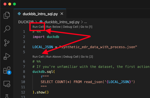
Fig. 1 – How to run a cell in VSCode notebooks
You can (re)run the blocks as often as you like, but you must run the first block to provide duckdb as a usable library and sell the LOCAL_JSON constant, which contains the name of the JSON file, for brevity of the SQL commands in Python.
# %%
import duckdb

LOCAL_JSON = "synthetic_edr_data_with_process.json"
The foundational SQL operation is using the SELECT statement, this is also known as the Data Query Language (DQL). You will always use SELECT in every query you execute. Additionally, you will always use the FROM statement, which is the target table or dataset that you are querying the data from.
In DuckDB, the read_json() operation is a DuckDB-specific function that enables you to consume and use JSON as a database within the engine. You could replace this with read_csv() or read_parquet() functions as well. For more information see the Importing Data section of the DuckDB documentation.
If you received a dataset you were unsure of the size and couldn’t gauge it easily from the logical size (kilobytes, megabytes, etc.), you can use the COUNT() function to return the specific amount of rows from a given criterion. Using the wildcard (*) inside of the COUNT() function will count all rows in the given dataset to give you an idea of how large of a dataset you are interacting with.
To execute SQL statements with DuckDB’s Python SDK, you use the duckdb.sql() function and pass the SQL query as a string. Using the show() method is what allows you to see the result set of your query. To put all of these concepts together, execute the following block to count how many rows are in the dataset.
AUTHOR’S NOTE: As an added learning challenge, use another dataset such as the CloudTrail logs from flaws.cloud or a dataset from your own environment, to practice with these concepts further.
# %%
duckdb.sql(
    f"""
    SELECT COUNT(*) FROM read_json('{LOCAL_JSON}')
    """
).show()
Limits and Uniqueness
Like in all things, moderation is key. Using COUNT(*) is an informative way to know how to limit yourself, in this case, using the LIMIT statement. LIMIT sets the maximum number of rows to retrieve from your dataset. As a human analyst, using LIMIT to reduce the amount of data viewed during your EDA can help prevent becoming overwhelmed as you learn the dataset.
As you apply more specific filtering and aggregation, the amount of rows returned will naturally reduce, but LIMIT can always be used as a fallback, or as an additional limiting factor. Execute the following block to retrieve all fields (again, using the wildcard) with a LIMIT of 10 rows.
# %%
duckdb.sql(
    f"""
    SELECT * FROM read_json('{LOCAL_JSON}')
    LIMIT 10
    """
).show()
To enforce row uniqueness, use the SELECT DISTINCT statement to return distinct (unique) values. This is helpful in certain cases to further reduce the amount of data returned, such as querying for unique instances of notables or indicators in a dataset. For example, retrieving the unique names of users in authentication logs, or the IPs or UUIDs of devices in an EDR dataset.
Additionally, SELECT DISTINCT can be leveraged to return unique values of highly repetitive logs such as AWS VPC Flow Logs or generic business application or network logs.
# %%
duckdb.sql(
    f"""
    SELECT DISTINCT * FROM read_json('{LOCAL_JSON}')
    LIMIT 10
    """
).show()
The SELECT DISTINCT statement becomes more impactful when specifying a small number of fields. In SQL you do this by providing a comma-separated list of the field (column) names. When dealing with nested data such as JSON objects and arrays in DuckDB, you use dot-notation such as in the jq CLI tool, where each level of hierarchy is period-separated.
In the following query, you can retrieve every unique pair of device IP addresses and the filename of the suspected malware sampled by the imaginary EDR tool. Modifying the statement by adding more fields demonstrates that your EDA can produce an overwhelming amount of results despite the distinctiveness.
# %%
duckdb.sql(
    f"""
    SELECT DISTINCT
        device.ip,
        file.name
    FROM read_json('{LOCAL_JSON}')
    LIMIT 10
    """
).show()
After running this block you may have noticed that the column names were truncated to the last value in the dot-notation, ip and name, respectively. This is the typical behavior of most SQL engines and can be remedied by creating aliases using the AS keyword.
The AS keyword will provide custom field names to make your EDA results more readable, or to maintain the context of deeply-nested data within your dataset. The AS keyword can also be used to output complex calculations and functions from more advanced SQL functions and clauses into an aggregatable field.
# %%
duckdb.sql(
    f"""
    SELECT DISTINCT
        device.ip AS device_ip,
        file.name AS file_name
    FROM read_json('{LOCAL_JSON}')
    LIMIT 10
    """
).show()
Finally, mathematical and statistical operators such as COUNT() can be combined with the SELECT DISTINCT statement to provide a total of distinct values. This can further inform the total number of rows to be used within LIMIT statements or be used as an overly simplistic aggregation mechanism.
In the case of this dataset, there is total uniqueness across both IPs and filenames in that the distinct count of both device IP addresses and file names are 1000.
# %%
duckdb.sql(
    f"""
    SELECT DISTINCT
        COUNT(device.ip) as total_device_ips,
        COUNT(file.name) as total_file_names
    FROM read_json('{LOCAL_JSON}')
    """
).show()
Congratulations, you have successfully mastered the basics of SQL. There is a lot of value that can be derived from datasets using simple operators such as COUNT(), specifying field names, and using basic statements such as AS and SELECT DISTINCT. In the next section, you will learn more advanced aggregate functions.
Aggregating and Filtering
While SELECT DISTINCT can be used for very simple aggregations, it is too rigid for meaningful aggregation across a large number of fields. A simple type of aggregation is grouping a specific field alongside the amount of times the values within that field are present in the dataset.
For example, you can use this to find the “top 10” or “top 100” hostnames, IP addresses, or device owners implicated in the EDR findings. You could further use this style of aggregation to find the amount of times a user agent appears in network logs, the largest share of User Principal Names (UPNs) appearing in Microsoft Defender XDR or EntraID logs, or the “top callers” to your honeypot.
To start an aggregation, specify a field by its name and then again using the COUNT() function and AS statement to create an alias. Then, use the GROUP BY statement to group rows of the same values into “summary rows”. In this case, you are creating an aggregation of the amount of times device IPs appear in the dataset.
To numerically order and stack rank the aggregation, use the ORDER BY keyword along with the field name to sort on, and a direction: either ascending (ASC) or descending (DESC). The clause ORDER BY total_device_ips DESC orders the resulting aggregation descending from the highest value of occurrence of the IP. The LIMIT statement is used for brevity.
# %%
duckdb.sql(
    f"""
    SELECT
        COUNT(device.ip) AS total_device_ips,
        device.ip AS device_ip
    FROM read_json('{LOCAL_JSON}')
    GROUP BY device_ip
    ORDER BY total_device_ips DESC
    LIMIT 15
    """
).show()
To filter on specific values within a dataset using SQL, you use the WHERE clause to extract a specific (or several) row that only matches the condition in the WHERE clause. This is also known as a SQL predicate, which is defined as a “condition expression that evaluates to true or false”. Another way to consider this concept is that the WHERE clause is only returning rows where the value of a field is present, or a boolean “True”.
The simplest type of filtering with WHERE is an equality search. This can be used to query for results where an indicator or notable matches a specific value, or where the normalized severity or common values such as a status, Traffic Light Protocol (TLP), or activity match a given condition. In this case, you are querying for a specific device IP in the EDR dataset. Feel free to rewrite the predicate to search for other values.
# %%
duckdb.sql(
    f"""
    SELECT DISTINCT
        *
    FROM read_json('{LOCAL_JSON}')
    WHERE device.ip = '188.166.30.169'
    """
).show()
Multiple filters can be specified in the WHERE clause by using SQL boolean operators AND and OR. Predicates can contain multiple AND and OR to apply greater conditional control over your filter.
This can be useful for providing a handful of extra values for a predicate or to match across multiple matching criteria, such as finding high severity alerts in a dataset that implicates a specific user with a specific role or is identified as an administrator.
In the following example, several fields are requested from the EDR data: hostnames, usernames, SHA-256 hashes, file paths, and file names. These fields are only returned where the normalized severity is fatal or critical and the EDR finding is actively being worked (“In Progress”).
# %%
duckdb.sql(
    f"""
    SELECT DISTINCT
        device.hostname AS hostname,
        device.owner.name AS username,
        file.sha256_hASh_data.value AS sha256,
        file.path AS file_path,
        file.name AS filename
    FROM read_json('{LOCAL_JSON}')
    WHERE severity = 'Fatal'
    OR severity = 'Critical'
    AND status = 'In Progress'
    """
).show()
This filtering can be combined with even more functions such as COUNT(), if you were performing a less specific audit to retrieve the total amount of specific events in a dataset. For instance, finding the total amount of findings that are fatal or critical severity and are in progress.
# %%
duckdb.sql(
    f"""
    SELECT DISTINCT
        COUNT(*) AS total_matching_findings
    FROM read_json('{LOCAL_JSON}')
    WHERE severity = 'Fatal'
    OR severity = 'Critical'
    AND status = 'In Progress'
    """
).show()
Alternatively, as demonstrated earlier, use aggregates instead of predicates to perform that same type of analysis without the specificity. Practice using different fields in the ORDER BY clause to further organize the data in meaningful ways.
This aggregation can be used in visualization libraries such as matplotlib or xarray and also exported to CSV files to create charts in PowerPoint or external business intelligence (BI) tools.
# %%
duckdb.sql(
    f"""
    SELECT DISTINCT
        severity,
        status,
        COUNT(*) AS alert_COUNT
    FROM read_json('{LOCAL_JSON}')
    GROUP BY severity, severity_id, status
    ORDER BY alert_COUNT DESC
    """
).show()
Finally, conditional logic can be applied into aggregations by using the HAVING clause which provides the filtering control similar to the WHERE clause, but is able to be used within aggregations for even more specific filtering.
For instance, you can use the WHERE clause for gross filtering adjustments such as filtering on the normalized values of status, severity, activity, or otherwise, and utilize the HAVING clause to filter aggregation-specific values such as the amount of occurrences of an IP address or other indicator. You can also use the HAVING clause to filter devices that breach a certain threshold of alerts as demonstrated in the script block below.
# %%
duckdb.sql(
    f"""
    SELECT
        device.hostname AS host,
        device.type AS device_type,
        COUNT(*) AS alert_count
    FROM read_json('{LOCAL_JSON}')
    WHERE status != 'Suppressed'    GROUP BY device.hostname, device.type
    HAVING alert_count > 3
    """
).show()
In this section, you learned how to further aggregate and sort your EDA results using the GROUP BY statement and ORDER BY clause. Additionally, you learned to filter your dataset using the WHERE and HAVING clauses for basic filtering, and aggregate-specific filtering, respectively. Finally you learned how to combine multiple filters within a predicate by using the boolean OR and AND operators. In the next section, you will learn how to work with timestamps in SQL and how to extend your filtering with basic pattern matching.
Timestamps and Pattern Matching
Working with timestamps as an analyst – SecOps or not – is absolutely essential, and also soul-crushing. There are several types of specifications of timestamps that can be written in different ways. Timestamps have specific data types in different coding languages, have different formats (RFC3389, ISO-8061, Apache Log, etc.), and never seem to match your timezone or precision.
Thankfully, since this is a blog, your soul will not be crushed. If there are ample requests from the community, we will author another blog on working with time in SQL with greater utility.
While this dataset only covers ~36 hours of events, there is still utility in separating results by specific intervals of time. For instance, you can truncate the timestamps into yearly, monthly, daily, and/or hourly intervals. This can be used with an EDA to quickly assess the seasonality of data or any specific outliers within a given time interval. This can be helpful for customer-facing systems, for spotting network flood attacks, or just for benchmarking traffic.
To truncate by intervals, you must have a valid TIMESTAMP SQL data type in your dataset. Next, use the DATE_TRUNC() function to specify the interval and the timestamp field to create the truncation on. In this example you are creating an aggregation on the alerts-per-hour that are not suppressed, ranked by the amount of alerts per hour truncation. You can replace hour with day` for an even smaller time-truncated aggregation.
Which hour has the most findings? Which has the least? If this was a real example, what would you expect to see in your organization?
# %%
duckdb.sql(
    f"""
    SELECT
        COUNT(*) AS alert_count,
        DATE_TRUNC('hour', time) AS event_hour
    FROM read_json('{LOCAL_JSON}')
    WHERE status != 'Suppressed'
    GROUP BY event_hour
    ORDER BY alert_count DESC
    """
).show()
An additional way to perform time-based analysis is using the EXTRACT() function to extract specific interval components from a timestamp, such as the specific hours, days, months, and/or years. Instead of having a truncated timestamp as the aliased field values, you will have the extracted integer. This may aid in readability and/or utility depending on the use case.
In the following example, EXTRACT() is used to pull the day, month, and year components into the aggregation instead of the hourly aggregation example you executed previously.
# %%
duckdb.sql(
    f"""
    SELECT
        EXTRACT(day FROM time) AS event_day,
        EXTRACT(month FROM time) AS event_month,
        EXTRACT(year FROM time) AS event_year,
        COUNT(*) AS alert_count
    FROM read_json('{LOCAL_JSON}')
    WHERE status != 'Suppressed'
    GROUP BY event_day, event_month, event_year
    ORDER BY event_day DESC
    """
).show()
Lastly, stepping back from working with timestamps, you can further refine your EDA skills by using fuzzy matching with the LIKE operator in the WHERE clause. This LIKE operator is one of four mechanisms for pattern matching with DuckDB. For more information refer to the Pattern Matching section of the DuckDB documentation.
The LIKE operator on its own will behave like an equals operator without the usage of special symbols. The underscore (_) character matches any single character, and the percent sign (%) matches any sequence of zero or more characters. For example, refer to the following SQL examples from the DuckDB documentation showing how the LIKE operator functions. The true comments denote a match.
SELECT 'abc' LIKE 'abc'; -- true
SELECT 'abc' LIKE 'a%' ; -- true
SELECT 'abc' LIKE '_b_'; -- true
SELECT 'abc' LIKE 'c';   -- false
SELECT 'abc' LIKE 'c%' ; -- false
SELECT 'abc' LIKE '%c';  -- true
SELECT 'abc' NOT LIKE '%c'; -- false
When the percent sign is used in front of the string, the LIKE operator behaves like an “ends with” operator, such as WHERE device.owner.email_addr LIKE ‘%gmail.com’. This will search for email addresses that end with “gmail.com”. This pattern can be used for searching for specific last names, domains in email addresses, or any other context-specific data appended to a string.
When the percent sign is used behind the string, the LIKE operator behaves like a “starts with” operator, such as WHERE device.name LIKE ‘centos%’. This will search for any devices that begin with “centos” which would potentially denote an asset with the CentOS Linux distribution installed. This pattern can be used for similar tasks where an appended value to a string has contextual meaningfulness or when looking for specific directories or command line arguments in other values.
Lastly, when percent signs are used on both sides of the string, the LIKE operator behaves like a “contains” operator, such as WHERE metadata.product.vendor_name LIKE ‘%Mashino%’. This will search for logs where the vendor names contain Mashino, in a case sensitive manner. All operations with the LIKE operator are case sensitive. This is the string pattern matching operation with the most “gross adjustment”.
How would you use these different wildcards in your day to day job? Is there a time where you would prefer to use starts with over contains? Would you use ends with over contains? Would you always opt for “contains” style searches or would you prefer strict equality matching?
In the following example, you’re retrieving asset and potential malware file names in the EDR dataset where ssh is in the filepath. This can denote malware that was downloaded via a remote SSH session, or the SSH session was opened to a forward-staged Command & Control (C2) node to retrieve the malware. Using LIKE and pattern matching can prove helpful in hunting for specific tradecraft and can be used to add further specification to aggregations.
# %%
duckdb.sql(
    f"""
    SELECT
        device.hostname AS hostname,
        device.ip AS device_ip,
        device.agent.uid AS agent_id,
        file.name AS filename
    FROM read_json('{LOCAL_JSON}')
    WHERE file.path LIKE '%ssh%'
    ORDER BY hostname ASC
    """
).show()
Lastly, the LIKE operator can be negated using the NOT operator. Negation is also known as an “opposite” operator. This can be helpful when there are three or more values and you want to exclude a single one, or when there is a large number of results and you want to specifically negate a few. It can be faster to utilize negation versus equality operators with several OR boolean operators.
For pattern matching in an even less precise manner, consider the ILIKE operator which is the case-insensitive version of the LIKE operator. This is helpful when you do not know the casing over specific values in the dataset or where there is inconsistency in casing, this can be applicable to various indicators and notables or other file system and network-specific data points.
The following example uses both negation (NOT LIKE) and case insensitive pattern matching (ILIKE) to further filter the EDR dataset. In this case, any paths that start with “C” – such as in a Windows operating system – are excluded, but any MITRE Technique name that mentions “shadow” are included in the search. This is not the best practical demonstration, could you find a better way to use negation or case insensitivity?
# %%
duckdb.sql(
    f"""
    SELECT
        device.hostname AS hostname,
        device.ip AS device_ip,
        device.agent.uid AS agent_id,
        file.name AS filename
    FROM read_json('{LOCAL_JSON}')
    WHERE file.path NOT LIKE '%C%'
    AND finding_info.attack_technique.name ILIKE '%shadow%'
    ORDER BY hostname ASC
    """
).show()
In this section you learned how to work with timestamps as part of aggregations using the DATE_TRUNC() and EXTRACT() functions to truncate and pull time components out of valid timestamps, respectively. You also learned how to perform fuzzy pattern matching using the LIKE and ILIKE operators in your predicates for “contains” style searches. Finally, you learned how to use negation with the NOT operator for a different style of search. In the next section you will learn how to apply specialized conditional logic to your queries, work with null data points, statistics, and perform very rudimentary trend analysis.
Conditional Logic, Statistics, and Trend Analysis
Working with aggregations is good to group data points together for an investigation or an audit. However, you may have situations where limited data transformation can prove beneficial, such as providing a custom label based on the combinations of data you’re searching for in your predicate. For example, you may want to generate a label to denote impact, severity, and/or risk levels based on other field values inside of the dataset.
You can achieve this conditional logic with the CASE expression, which operates similarly to an if-then-else statement, such as an if, elif, and else conditional loop in Python. For more details on the DuckDB-specific implementation, refer to the CASE Statement section of the DuckDB documentation.
The CASE expression has several uses beyond conditional logic for filtering. You can also use the CASE expression to perform conditional updates to a database, called an “upsert”, and conditional deletions as well. This can be useful when updating a specific incident or finding within a database or data lake, however, these specifics are out of scope for this blog.
To use the CASE expression, conditions are specified using the WHEN clause, which is similar to using the WHERE or HAVING clauses. Boolean operators AND and OR can be used within the WHEN clause to create compound conditions. Finally, the THEN clause defines your action, or the value you want to create.
To catch any other non-matching conditions, use the ELSE clause. Without using it, any non-matching conditions will be returned as nulls instead of as a boolean false. To close the CASE expression use the END keyword, which can be aliased using the AS keyword to contain values defined by the THEN clause. This can be used to bring the value as a field name for aggregations with the GROUP BY statement.
In the following example, you are creating a notional impact_level field using a CASE expression based on the specific version of the CentOS Linux distribution installed on a device. Whenever you reference fields in the CASE expression they must also be included in the GROUP BY statement.
# %%
duckdb.sql(
    f"""
    SELECT DISTINCT
        device.hostname AS hostname,
        device.ip AS device_ip,
        CASE
            WHEN device.os.name = 'CentOS' AND device.os.version = '8' THEN 'High Impact'
            WHEN device.os.name = 'CentOS' AND device.os.version = '8.2' THEN 'Medium Impact'
            WHEN device.os.name = 'CentOS' AND device.os.version = '9' THEN 'Low Impact'
            ELSE 'No Impact'
        END AS impact_level
    FROM read_json('{LOCAL_JSON}')
    WHERE device.os.name = 'CentOS'
    GROUP BY device.hostname, device.ip, device.os.name, device.os.version
    ORDER BY hostname ASC
    """
).show()
Multiple CASE expressions can be used within a query, but be wary of any performance penalization when attempting to use these in OLTP workloads or within query engines for data lakes such as Amazon Athena. This is where using DuckDB shines given its vectorized-columnar query engine, but note that this is also an incredibly small dataset.
When working with security and IT observability data, it is not uncommon to have several nulls within the dataset. This can be by design of a source system that will not provide certain key value pairs due to specific conditions, or general incompleteness of data due to data transformation efforts or sampling.
To avoid nulls inside of aggregations, or to otherwise provide a placeholder value for nulls, similar to the previous CASE expression example – consider using the COALESCE() function. The COALESCE() function can take any number of arguments, such as field names, and returns the first non-null value that it finds. Similar to the CASE expressions ELSE clause, you can provide a “fallback” value if all other arguments are returning null.
For instance, take a situation where authentication logs from a device in Microsoft can capture the User Principal Name (UPN), the Security ID (SID), the username, and the Object ID. Some or all of these may be null. You can use COALESCE() to return the first value that is not a null, or create your own value. This can be used for spot-checking data completeness during an EDA or to create more conditional friendly values.
In the following example, the COALESCE() function is used similarly to the example case above, filling in a value when all of the identifiers within device.owner JSON object are null.
# %%
duckdb.sql(
    f"""
    SELECT DISTINCT
        device.hostname AS hostname,
        COALESCE(device.owner.uid, device.owner.email_addr, device.owner.domain, 'Unknown') AS device_owner
    FROM read_json('{LOCAL_JSON}')
    ORDER BY hostname ASC
    """
).show()
Calling back to the earlier sections when you used the COUNT() function, there are other statistical functions that exist within SQL that can be used. For instance, the AVG(), MAX(), and MIN() functions are used to gather average, maximum, and/or minimum values of integers, or float data types within a dataset, respectively. These statistical values can further be aliased and used within aggregate functions as well.
The usage for statistical functions in SQL during an EDA can be useful for the assessment of login frequencies, of the amount of time a specific host is connected to from a given source, or to use as the basis for simple anomaly detection in network, file system, process, or identity logging sources. You can combine several of these together to create averages of the count of certain fields in your logs to generate an integer to work with.
In the following example, the normalized values of risk and severity are used in the various statistical functions. This wouldn’t be the best use case, but MIN() and MAX() functions can be used to determine the extreme upper and outer bounds of a field’s value.
# %%
duckdb.sql(
    f"""
    SELECT
        AVG(risk_level_id) AS avg_risk,
        AVG(severity_id) AS avg_sev,
        MAX(risk_level_id) AS max_risk,
        MAX(severity_id) AS max_sev,
        MIN(risk_level_id) AS min_risk,
        MIN(severity_id) AS min_sev
    FROM read_json('{LOCAL_JSON}')
    """
).show()
To finish off the introductory EDA tutorial, the last functions to briefly cover are window functions, which allow you to perform calculations across a specific row of data while maintaining visibility of the other rows. Stated differently, window functions allow you to “zoom into” each event while seeing the bigger picture or themes of all other events around them, as they don’t use “summary rows” like with the GROUP BY clause.
For instance, you can use window functions to show how failed login attempts fit in with attempts of specific users or IP addresses. It is useful for identifying potential anomalies or at least to spot trends during an EDA. For more information about window functions in DuckDB and general examples refer to the Window Functions section of the DuckDB documentation.
Window functions are different from aggregate functions, such as GROUP BY paired with the COUNT() and/or AVG() functions, because GROUP BY collapses the rows into a summary row – as you have demonstrated multiple times – so you lose context of an individual event. Window functions do not organize the data into summary rows, so you retain any granular insights while looking at specific event-to-event or events-over-time comparisons.
One type of window function is the ROW_NUMBER() function that assigns unique, sequential values to each row in a result set, starting from 1. This is beneficial for creating a ranking of rows, and it can be partnered with another SQL clause, PARTITION BY. Partitions are groups of rows that allow you to view them and perform computation operations on the subset of partitions.
Partitions are also a table creation and management strategy for performance management by only writing queries against specific data stored in certain partitions. This is covered in our Amazon Athena and Apache Iceberg for Your SecDataOps Journey blog in much greater detail, and is out of scope for this blog.
Using ROW_NUMBER() with partitions allows you to stack rank the groups of data points in the partition. You can partition by time or by any shared, common value within a specified field for the partition. For instance, you can group by user, device, finding category, activity, actions, severity, or status. As mentioned above, you do not lose the context of the events that match your query, as they are not stored in a summary row.
To use ROW_NUMBER() you partner it with the OVER() clause that defines the actual window of the window function. Using PARTITION BY is optional, but you should use ORDER BY to sort the windowing function. In the SQL query below, you are requesting several fields of note from the EDR dataset and setting the window function over file name, based partitions ordered by event time. Like other SQL functions, the output can be aliased using the AS keyword and further utilized in another ORDER BY clause.
# %%
duckdb.sql(
    f"""
    SELECT DISTINCT
        device.hostname AS hostname,
        finding_info.title as finding_title,
        finding_info.attack_technique.uid as attack_technique_id,
        file.name as filename,
        ROW_NUMBER() OVER (
            PARTITION BY
                file.name
                ORDER BY time
        ) AS malware_count
    FROM read_json('{LOCAL_JSON}')
    ORDER BY malware_count DESC
    """
).show()
The result set demonstrates the value of keeping individual rows instead of several aggregations when using GROUP BY if maintaining the original context during the EDA was important. How else would you implement partitions for this window function? What other times would you utilize a window function over an aggregate function, and vice versa?
In this section you learned how to implement conditional if/else logic using the CASE expression as well as the COALESCE() function while also handling null values with the latter. You learned how to use other basic statistical functions such as AVG(), MIN(), and MAX(), and how they could be partnered with the COUNT() function. Finally, you learned how to use the ROW_NUMBER() window function and PARTITION BY clause to create aggregations over actual rows of data and not just summary rows.
Conclusion
In this blog you learned how valuable performing Exploratory Data Analysis with SQL can be as a security operations analyst or other security specialist. You learned how to use DuckDB, an in-memory vectorized analytical database, to execute SQL statements against semi-structured data stored in JSON files. Finally, you learned how to implement over a dozen different SQL functions, statements, operations, and clauses for working with various data points and data types.
While longer term success of a SecDataOps program may rely on the usage of big data and analytics query engines and storage solutions within data warehouses and data lakes, EDA will always have its spot. Whether it is to perform quick threat hunts, to enable decision making as part of an internal investigation or incident response, or to perform audits of otherwise well-structured and normalized security and IT observability data, using EDA to process datasets is essential for successful security practitioners. Writing SQL and learning how to expand your EDA skill sets can prove to be an operational and tactical boon for harnessing data and making it work for you.
Query’s Federated Search platform can also help with EDA across several 100’s of datasets in a federated manner. Instead of working with one dataset, you can work across multiple data lakes, log analytics platforms, SIEMs, warehouses, and direct APIs without needing to learn SQL, or another other query language. If that is of interest to you, feel free to book a demo with yours truly or one of our customer success managers or account executives.
This is the first of hopefully many more shorter hands-on blogs centered on EDA. If you want to be called out or otherwise featured in the next entry please share your own queries – which can use functions and clauses you learned here, or not – and we’ll pick a dozen or so to include in our next blog! Until next time…
Stay Dangerous.