In our previous blogs on Artificial Intelligence and Everyday Life, we learned the basics of how our computers can be trained to think like humans and work like them. Now let’s move on to some actual application of what we learned and understand about one of the most versatile neural network models – The Autoencoder.

Let’s look at the formal definition of an Autoencoder before we try to understand it in depth.
“An autoencoder is a type of artificial neural network used to learn efficient data codings in an unsupervised manner. The aim of an autoencoder is to learn a representation for a set of data, typically for dimensionality reduction, by training the network to ignore signal “noise”. ” (https://en.wikipedia.org/wiki/Autoencoder)
You don’t need to scratch your head if you didn’t get it yet, because even I didn’t! So now let’s break this down for you.
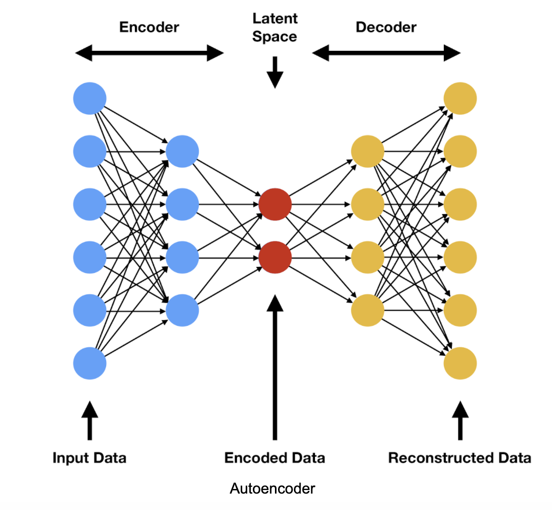
An Autoencoder is an Unsupervised model, which means that we don’t need to feed it any ‘labeled’ data. If you look at the above representation of an autoencoder, you might have noticed it’s symmetric structure, which explains to a large extent how it works. As per the definition, the primary use of an autoencoder is for dimensionality reduction. Dimensionality reduction is the process of retaining only the essential features in a dataset. You could be wondering: how can I use it for anomaly detection? To understand this, we need to understand the latter part of its definition: how it’s trained to ignore ‘noise’.
Let’s have a look at some of the salient features of an Autoencoder before moving on to its working.
- Input & Output layers are Identical
- Lesser number of nodes in the hidden layers (inner layers)
- Retains only the important features while encoding
- The output is the recreated data
Working of an Autoencoder for Anomaly Detection
First, add the training input data into a newly created autoencoder. This process is just a simple neural network with the above architecture.
Next, the autoencoder ‘compresses’ the data through the process of dimensionality reduction. ‘Compressing’ the data means it retains only the essential and most prominent features in the data set. Solely these values are provided to the output layer forming the reconstructed data. Now to get rid of the ‘noise,’ or the non-essential or less-occurring features in the dataset, we train the model.
Lastly, feed the test dataset into this trained model. Then compare the output of this model with the actual input data, which gives us the amount of noise present in the test dataset. The higher the amount of noise, the higher the probability of an anomaly in the dataset!
Here’s a real-life example of how our brain uses this autoencoding process for anomaly detection too!
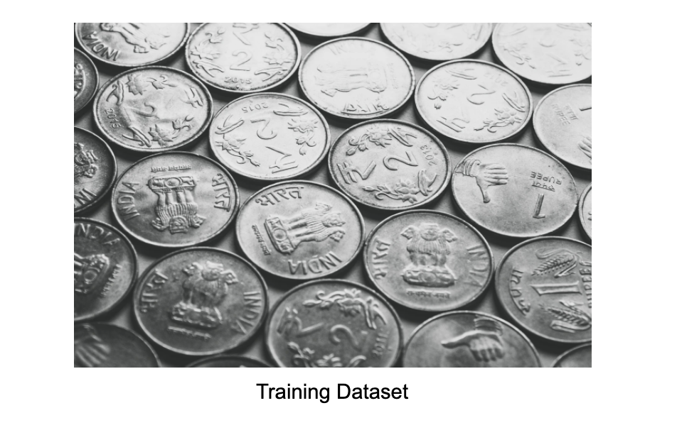
The most straightforward application of anomaly detection could be while searching for something in a large dataset. Suppose I have a bag of coins which contains identical coins of type A and B. This is my training data for the autoencoder in our brain. The coins may be old or new, polished, or tarnished or even having a unique identification number in some cases. Still, our minds wouldn’t retain all such features but will remember a select few, like the size, color, the emblem, patterns on it, etc.


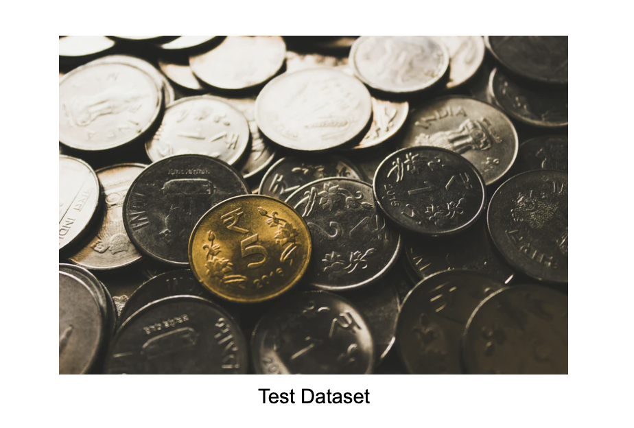
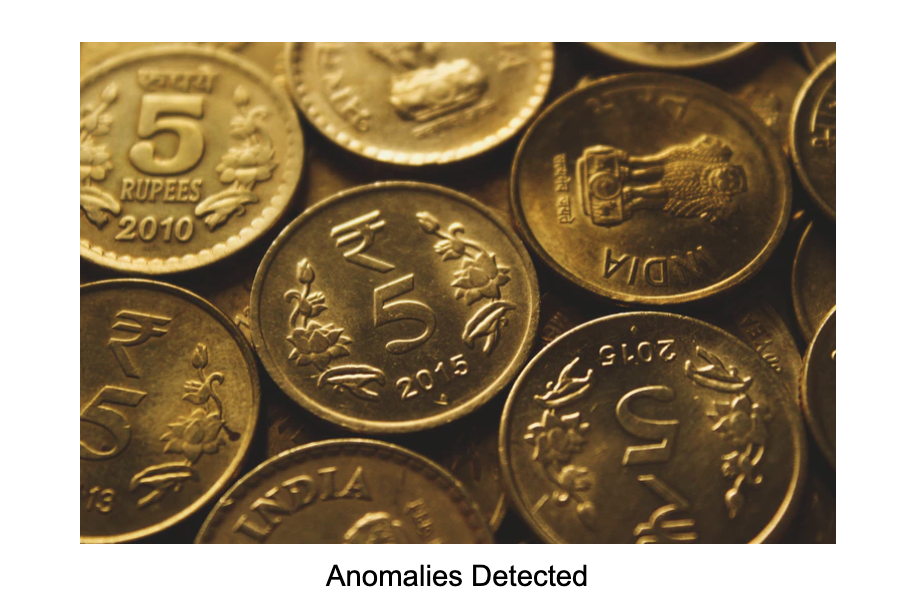
Now suppose we get our test dataset in the form of another bag which has coins of type A and B mixed with another type of coins C. So how would we remove these anomalous coins of type C from this bag? We would look at each coin and try to match it with the features we remember from our ‘training’ set. The critical thing to note here is that we wouldn’t look at all the details of a coin, but only those features we remember from our past experience. If we observe a variation (noise) in these features, we classify those coins as anomalies. Tada! That’s how the autoencoder inside our brain works.

While we just explored Anomaly Detection as one of the uses of this model, look for its other applications such as Dimensionality Reduction, Information Retrieval, and Machine Translation, etc.
Did you enjoy this content? Follow our linkedin page!


