
This is part 4 of this series on Data Analysis. The focus of this article is how to take raw data and make it more suitable for analysis.
Datasets we want to analyze are rarely perfect with no typos, missing values, or outliers. These things can all affect the results of our analysis, and we must take the time to look at these things and take steps to alleviate the problem.
Data cleaning or cleansing is the process of identifying and handling inaccurate, unreliable, or irrelevant entries in a data set. There are lots of techniques for data cleaning, and we won’t get into them all here; however, we will cover the basics.
The first step is understanding what needs cleaning. Identifying problems in the data can be difficult. Some common things to look for are extra spaces in between words, inconsistent capitalization, missing values, numeric data that is stored as text, duplicate rows, spelling errors, mismatched columns. This can be a very complicated process but will result in more accurate results.
As an example, we can walk through some potential problems with the titanic data set that we have been using from Kaggle. The first step is to look at the overall structure of the data set. This is done with the following python command, where ‘train’ is the variable where I have stored my dataset as a pandas data frame.
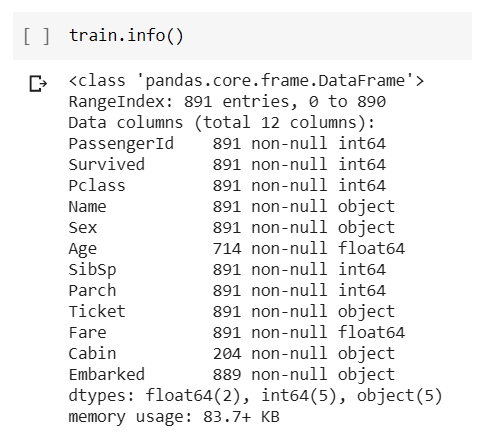
From the output, we can see that our data has 891 rows (numbered 0 to 890) and 12 columns. This is an excellent way to double-check that our values are stored in a data type that makes sense. All the values that should be numeric, should be stored in a numeric data type. Everything in this data set seems to be okay.
A simple thing to check for is duplicated rows.
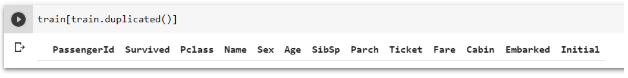
Our data set doesn’t have any duplicated values.
Another thing we can check is for uniformity of the values in the data set. This command provides a broad overview of the general shape of the values in the data set.
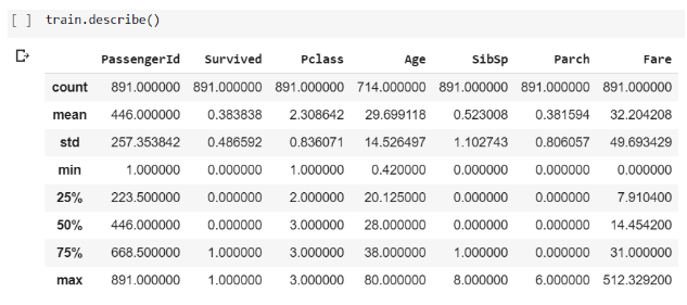
From before, you’ll remember that we found that our data has 891 rows. In this table, you can see how many entries are in each column. Every column appears to be full except for the Age column, which looks like it’s missing a lot of values (more on that later). Another thing to notice in this table is that some of the statistics don’t make any sense. The “PassengerId” column is just a column that counts from 0 to 890 to give each passenger and unique identifier. Taking the mean of that doesn’t make any sense analytically. The “Survived” column is a 0 for people who did not survive the titanic and a 1 for people who did. Taking the mean of that doesn’t mean anything significant. Another thing you might notice is that this command only gave us information about the numeric columns. We did not include all column values.
We already noticed that the age column is missing values. Maybe some of the other non-numeric columns are missing data points too. We can look at this with this command.
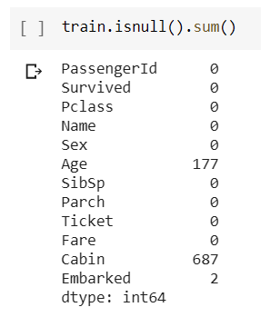
The Cabin column is missing 687 values. That’s over half of our rows. While there are different ways to handle this, I think our best option is to remove that column from our analysis. It’s hard to make any conclusions about it when over half the data is missing.
The most obvious issue in our data set is the massive amount of missing data in the Age column. Let’s look a little more at that column. From the table above, we can see that the average age of people on the ship is 29.7. The youngest person is 0.42, and the oldest is 80. A common thing to do is fill in all missing values with the average. So, all 177 people with missing ages would be assumed to be 29.7 years old. This would maintain the average age of people on the ship. There are ways to make it slightly more specific. Let’s see if we can make a correlation between another column and the age column. If we look at the first few rows of the data, we can get a better idea for what specific values look like:
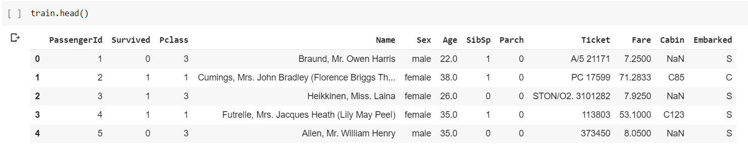
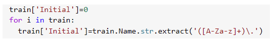
Notice that the ‘Name’ column contains a prefix (like Mrs., Ms., Mr., etc.). By using those values, we can find a better way to fill in the age column. I can create a new column names ‘Initial’ to store all of the prefixes.
From here, we can look at the average age of each type of person. 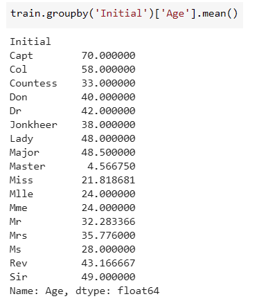
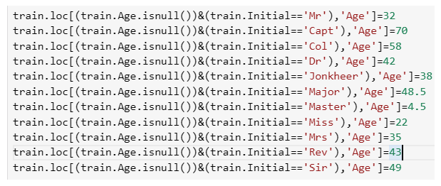
Maybe using this data, we could fill in the missing values a little more accurately. So, now, the entry on line 161, Master Thomas Henry Sage, will have an age of 4.566750 instead of 29. That might make a big difference in determining whether or not he survives. Doing a little rounding, we can use these commands to fill in these missing ages.
Now, if we look at our train info again, we can see that things look a little better.

We no longer have any missing values, and our mean age didn’t change too much. I would say this was a successful cleaning of the data. There are many more steps one could take to ensure the highest quality data, but this was a great example of a simple data clean.
Part 5: Data Classification, Clustering, and Regression will be available next Thursday, March 5. In the meantime, follow our linkedin page for more great content!